Artwork Categorization
Abdullah Ahmed, Alec Albrecht, Carlos Hernandez, Ankita Somu, Sanjana Srinivasan

Midterm Report
Link to the model codebase on Google Colab
Introduction/Background
With the rise of artwork generated by text-to-image models like DALL-E and Midjourney, it raises an interesting question about influences from source material. Generative art models are trained on large datasets including works from different art movements over time. Our team seeks to develop a solution for classifying an art piece into a stylistic period. This categorization algorithm could be used to identify and retrace the art styles mimicked in generative art. Previous approaches have used k-Nearest Neighbor and support vector machine algorithms to build their models (Falomir, Zoe, et al.).
Problem definition
Given an image our project aims to classify the style of an art piece. Our goal is to create a model that consistently classifies the style of the images in any collection.
Data collection
We are using a collection of artwork on Kaggle called the Best Artworks of All Time to train our model. The dataset identifies stylistic periods for each artist included in the collection. Our model will learn to categorize artwork to its respective artist based on its training data. The model will then be able to report what artist is most likely associated with a new artwork and then a stylistic period can be concluded.
Methods
Preprocessing
The preprocessing for the images from the dataset:
- Min-Crop to (x, x) dimensions where x = min(width, height)
- Resized to the minimum size of all images: (204, 204)
- Normalized to mean and standard deviation of the ImageNet dataset
- If the number of images per artist is less than 400, transform and clone the images by:
- Flip from left to right
- Flip from top to bottom
- Rotate 90 degrees
- Rotate 180 degrees
- Rotate 270 degrees
- Iterate until 400 image count is reached
- Finally, we randomly split our dataset into 85% training and 15% testing datasets
The purpose for the image transformations is to take care of classes in the dataset with a low number of data points. In our case, the artists Eugene Delacroix (31), Georges Seurat (43), Jackson Pollack (24) had low amounts of images in the dataset. These transformations allowed us to generate more data points for our model to train on.
Image Normalization


This is a showcase of how the image normalization changes the images. The histograms shown indicate a change in range from [0, 1] to a range centered around 0. The purpose of this normalization is to make the mean of all images 0 and the standard deviation of all images 1.
Metrics
Explaining our rationale for using certain metrics and how they are relevant to our model.
Loss vs Epoch
Loss is a common measure used to evaluate how well neural networks perform when working on training data. The loss shows the difference between the predicted outputs and the actual label values, which we should be minimizing to create an optimal model. The loss after each epoch should be decreasing throughout the training process. Visualizing and calculating how the loss changes after each epoch will give us a good idea of how successful the model is. Monitoring the loss vs. epoch will allow us to observe how the network is converging, and this value should rapidly decrease, as that would mean the model is adapting well to the training data, while a plateau in the graph may potentially indicate problems such as overfitting. This metric can also help us in improving our model, especially in terms of different hyperparameters (such as batch size or number of epochs), as we can see how changes in these may affect the loss, giving us ideas to fine tune. It will also assist in comparing both our models to see which one learns and converges better.
In a many of the DL frameworks like TensorFlow and PyTorch (used in our case), we optimize cross entropy loss and use that as a measure to see how efficient our implementation is. Because cross entropy is also logarithmic in nature, it gives us a very nuanced and precise way of measuring the accuracy of our model. Even a slight change can lead to significant drops in the deviations from the true distribution, which forces our model to be extremely accurate to get even moderately accurate predictions. This is relevant to our model because when we are analyzing paintings, we aim to reduce misclassification of genres and artists as much as possible. Especially in cases when we are trying to identify fraud, we must be overly particular in what similarity exists between the predicted and true distributions to give us the ground truth value. In essence, we will be working to get our cross entropy value as low as possible.
Confusion matrix
A confusion matrix is one of the most efficient ways to properly visualize how the model is performing for each artist batch specifically. Based on the batch that we want to sample, we can create True Positives, True Negatives, False Positives, and False Negatives categories and determine if the instances of a class are being correct or not, based on if they are in a class. Another reason we chose this is because we can measure the specificity rate, which is the true negative rate. We can thus measure the proportion of actual negative instances correctly predicted, and see if the model is biased toward predicting the majority vs minority classes. Finally, by analyzing TP, TN, FP, and FN, we know a confusion matrix is relevant to our model and the neural network system because it allows us to iteratively change the model to quickly identify misclassifications of identifying artists from paintings, which is not easily done with other metrics such as only looking at True Positives or area under the curve (detrimental for datasets that are imbalanced).
Model Architecture
Using PyTorch’s Neural Network class as a starting point, the architecture used for this dataset follows that proposed by Simonyan and Zisserman. Due to our image size, it consists of only 4 convolution layers each with a convolution, rectified linear unit (ReLU) and maxpool. The maxpool is always of size 2 and stride two, while the convolutions increase in number of filters, doubling from 64 to 512. Three fully connected layers and ReLUs step down the convolution output to the 50 classes in the data. Cross entropy loss is used to determine the loss for each batch and a stochastic gradient descent optimizer, also provided by PyTorch, was used for network backpropagation. A Batch size of 64 was used oer 25 epochs for initial training.
The testing dataset was then fed into the trained model. Since the output of the model is the vector of probabilities that a given image belongs to a particular class, the maximum value is taken as the predicted label. The accuracy of the model as a whole is calculated, as well as class specific accuracies defined as the number of labels correctly predicted out of the total size.
| Conv[3-64] | MaxPool | Conv[3-128] | MaxPool | Conv[3-256] | MaxPool => |
|---|---|---|---|---|---|
| 64x64x128x128 | 64x64x64x64 | 64x128x64x64 | 64x128x32x32 | 64x256x32x32 | 64x256x16x16 |
| => Conv[3-512] | MaxPool | Flatten | FC-4096 | FC-4096 | Fc-50 |
|---|---|---|---|---|---|
| 64x512x16x16 | 64x512x8x8 | 64x32768 | 64x4096 | 64x4096 | 64x50 |
Link to the model codebase on Google Colab
Results and discussion
General Results
So far, our model is quite successful, and is improving with adjustments. Without padding the dataset, the model had an overall accuracy of 19 percent, which is around 10 times better than random guesses, even though the specific accuracies for each class were not very high. After adjusting some hyperparameters such as the number of epochs and the batch sizes, the model improved significantly. 17 of the 50 artists were able to be classified with an accuracy of 50% or higher (all accuracies listed below), most probably the artists that had many images in the dataset. Many of the classes followed close behind, with accuracies in the high forties.
Model Accuracies by Class
| Artist Name | Percent Accuracy |
|---|---|
| Albrecht_Durer | 21.0% |
| Alfred_Sisley | 34.5% |
| Amedeo_Modigliani | 48.1% |
| Andrei_Rublev | 29.1% |
| Andy_Warhol | 69.2% |
| Camille_Pissarro | 42.0% |
| Caravaggio | 41.6% |
| Claude_Monet | 56.9% |
| Diego_Rivera | 51.1% |
| Diego_Velazquez | 53.5% |
| Edgar_Degas | 65.5% |
| Edouard_Manet | 46.4% |
| Edvard_Munch | 44.4% |
| El_Greco | 42.2% |
| Eugene_Delacroix | 52.5% |
| Francisco_Goya | 37.5% |
| Frida_Kahlo | 12.5% |
| Georges_Seurat | 38.6% |
| Giotto_di_Bondone | 52.6% |
| Gustav_Klimt | 43.1% |
| Gustave_Courbet | 52.7% |
| Henri_Matisse | 45.3% |
| Henri_Rousseau | 29.0% |
| Henri_de_Toulouse-Lautrec | 43.3% |
| Hieronymus_Bosch | 49.1% |
| Jackson_Pollock | 56.9% |
| Jan_van_Eyck | 86.4% |
| Joan_Miro | 23.4% |
| Kazimir_Malevich | 75.0% |
| Leonardo_da_Vinci | 59.6% |
| Marc_Chagall | 35.9% |
| Michelangelo | 40.6% |
| Mikhail_Vrubel | 41.4% |
| Pablo_Picasso | 28.1% |
| Paul_Cezanne | 39.3% |
| Paul_Gauguin | 25.9% |
| Paul_Klee | 49.1% |
| Peter_Paul_Rubens | 65.7% |
| Pierre-Auguste_Renoir | 50.0% |
| Piet_Mondrian | 23.2% |
| Pieter_Bruegel | 66.2% |
| Raphael | 31.1% |
| Rembrandt | 53.8% |
| Rene_Magritte | 14.1% |
| Salvador_Dali | 42.6% |
| Sandro_Botticelli | 68.7% |
| Titian | 20.0% |
| Vasiliy_Kandinskiy | 22.6% |
| Vincent_van_Gogh | 37.5% |
| William_Turner | 56.7% |
Loss vs Epoch
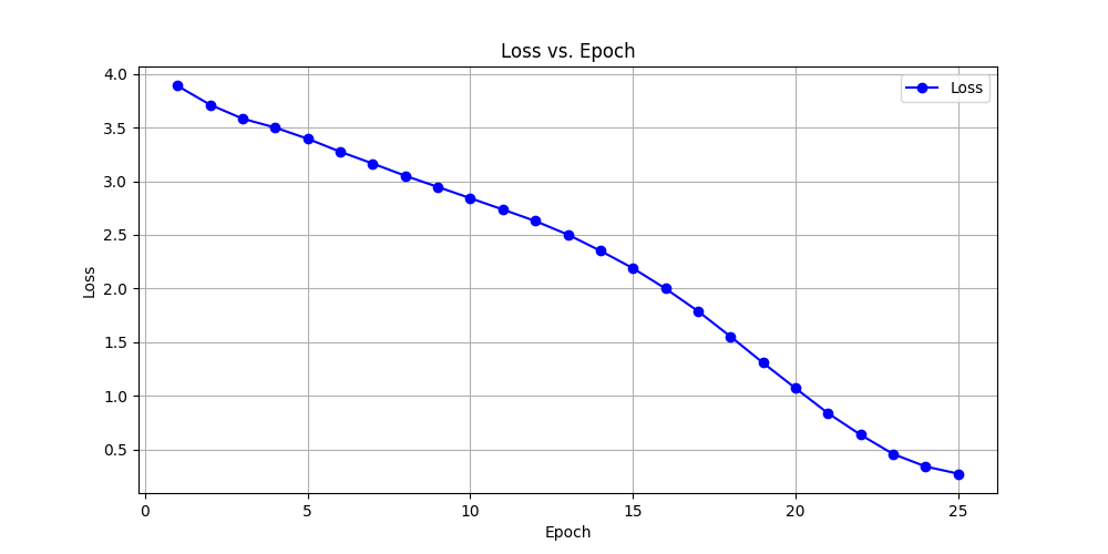
Analyzing our data, we know that our data points should be relatively logarithmic in nature and follow the opposite trend of a bell-curve, we attribute the lack of initial rise in our graphs to the fact that we are still working on training our model, and the batch size is still relatively unstable. For instance, the learning rate for our optimization algorithm is currently a bit low, so it is partially attributing to the slight plateau in the loss curve. Additionally, we are still experimenting with different batch sizes which will certainly impact the linearity of the loss curve.
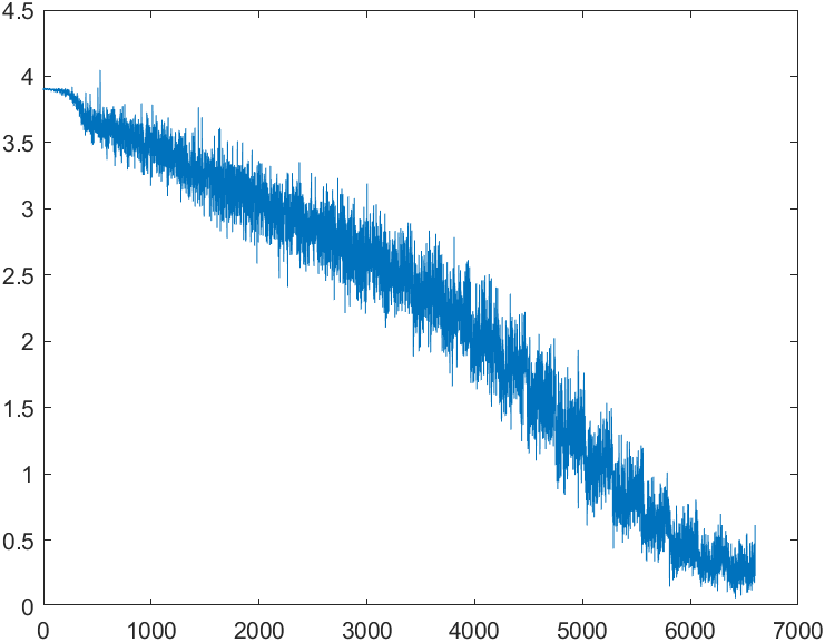 Loss trend across all batches
Confusion Matrix

The confusion matrix above depicts our predicted labels vs. the actual label values. The diagonal of the matrix represents the times that our model predicted the labels correctly, so ideally, the values on this diagonal should be high, and the values on all other positions in the matrix should be low, as these represent incorrect labeling from our model. Overall, the model appears to have a high accuracy, however there are some classes where the number of correct predictions is not as distinct from incorrect predictions for that class. However, there are rarely any classes for which incorrect predictions outnumber correct predictions. While the accuracy looks quite good, this is something that we can work to improve as we adjust our models, increasing our accuracy.
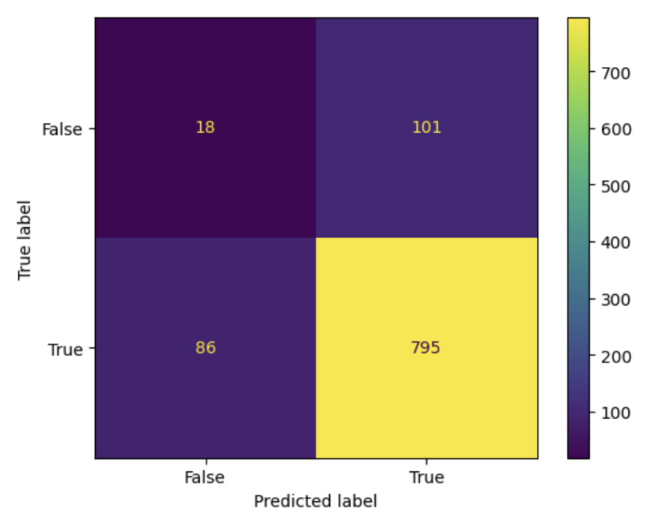 Confusion matrix preview of last batch
Precision, Recall and F1-Scores
| Artist Name | Precision | Recall | F1-Score |
|---|---|---|---|
| Albrecht_Durer | 0.32432432432432434 | 0.4528301886792453 | 0.37795275590551186 |
| Alfred_Sisley | 0.48717948717948717 | 0.31666666666666665 | 0.38383838383838376 |
| Amedeo_Modigliani | 0.2204724409448819 | 0.4666666666666667 | 0.29946524064171126 |
| Andrei_Rublev | 0.5217391304347826 | 0.2222222222222222 | 0.3116883116883117 |
| Andy_Warhol | 0.62 | 0.5535714285714286 | 0.5849056603773586 |
| Camille_Pissarro | 0.5490196078431373 | 0.25225225225225223 | 0.345679012 |
| Caravaggio | 0.5510204081632653 | 0.19852941176470587 | 0.29189189189189185 |
| Claude_Monet | 0.4782608695652174 | 0.18032786885245902 | 0.2619047619047619 |
| Diego_Rivera | 0.42105263157894735 | 0.38095238095238093 | 0.4 |
| Diego_Velazquez | 0.4393939393939394 | 0.48333333333333334 | 0.46031746031746035 |
| Edgar_Degas | 0.524390244 | 0.7166666666666667 | 0.6056338028169014 |
| Edouard_Manet | 0.31666666666666665 | 0.3333333333333333 | 0.3247863247863248 |
| Edvard_Munch | 0.4153846153846154 | 0.4909090909090909 | 0.45 |
| El_Greco | 0.6206896551724138 | 0.3103448275862069 | 0.41379310344827586 |
| Eugene_Delacroix | 0.49122807017543857 | 0.4827586206896552 | 0.4869565217391304 |
| Francisco_Goya | 0.5454545454545454 | 0.24 | 0.3333333333333333 |
| Frida_Kahlo | 0.23333333333333334 | 0.11864406779661017 | 0.15730337078651685 |
| Georges_Seurat | 0.36363636363636365 | 0.4827586206896552 | 0.4148148148148148 |
| Giotto_di_Bondone | 0.4868421052631579 | 0.6379310344827587 | 0.5522388059701493 |
| Gustav_Klimt | 0.38 | 0.3064516129032258 | 0.33928571428571425 |
| Gustave_Courbet | 0.31746031746031744 | 0.4 | 0.35398230088495575 |
| Henri_Matisse | 0.3717948717948718 | 0.5576923076923077 | 0.4461538461538461 |
| Henri_Rousseau | 0.4 | 0.14925373134328357 | 0.21739130434782608 |
| Henri_de_Toulouse-Lautrec | 0.28378378378378377 | 0.3 | 0.29166666666666663 |
| Hieronymus_Bosch | 0.4626865671641791 | 0.5166666666666667 | 0.4881889763779528 |
| Jackson_Pollock | 0.6268656716417911 | 0.5833333333333334 | 0.604316547 |
| Jan_van_Eyck | 0.8461538461538461 | 0.5789473684210527 | 0.6875 |
| Joan_Miro | 0.175 | 0.2 | 0.18666666666666665 |
| Kazimir_Malevich | 0.5084745762711864 | 0.6382978723404256 | 0.5660377358490567 |
| Leonardo_da_Vinci | 0.4125 | 0.5789473684210527 | 0.4817518248175182 |
| Marc_Chagall | 0.3684210526315789 | 0.2 | 0.25925925925925924 |
| Michelangelo | 0.3333333333333333 | 0.625 | 0.43478260869565216 |
| Mikhail_Vrubel | 0.272 | 0.5230769230769231 | 0.3578947368421053 |
| Pablo_Picasso | 0.5 | 0.14285714285714285 | 0.22222222222222224 |
| Paul_Cezanne | 0.5384615384615384 | 0.1 | 0.16867469879518074 |
| Paul_Gauguin | 0.20353982300884957 | 0.40350877192982454 | 0.27058823529411763 |
| Paul_Klee | 0.34545454545454546 | 0.3220338983050847 | 0.33333333333333326 |
| Peter_Paul_Rubens | 0.3148148148148148 | 0.25757575757575757 | 0.2833333333333333 |
| Pierre-Auguste_Renoir | 0.38095238095238093 | 0.38095238095238093 | 0.38095238095238093 |
| Piet_Mondrian | 0.21052631578947367 | 0.12698412698412698 | 0.15841584158415842 |
| Pieter_Bruegel | 0.4444444444444444 | 0.4745762711864407 | 0.4590163934426229 |
| Raphael | 0.21794871794871795 | 0.3953488372093023 | 0.2809917355371901 |
| Rembrandt | 0.7083333333333334 | 0.5573770491803278 | 0.6238532110091743 |
| Rene_Magritte | 0.21641791044776118 | 0.4393939393939394 | 0.29 |
| Salvador_Dali | 0.6206896551724138 | 0.5538461538461539 | 0.5853658536585366 |
| Sandro_Botticelli | 0.43820224719101125 | 0.8125 | 0.5693430656934307 |
| Titian | 0.2602739726027397 | 0.296875 | 0.2773722627737227 |
| Vasiliy_Kandinskiy | 0.3125 | 0.1724137931034483 | 0.22222222222222224 |
| Vincent_van_Gogh | 0.094339623 | 0.16666666666666666 | 0.12048192771084337 |
| William_Turner | 0.35526315789473684 | 0.4153846153846154 | 0.3829787234042554 |
| accuracy | 0.3796234028244788 | 0.3796234028244788 | 0.3796234028244788 |
| macro avg | 0.4106144987762023 | 0.3899332054177764 | 0.37601054370366105 |
| weighted avg | 0.4159938498220489 | 0.3796234028244788 | 0.371166493 |
We also reported metrics like precision and recall to calculate the f1-score. Precision is a measure of how many of the positive predictions are correct, in other words, how many TPs there are. On the other hand, recall is the number of positive cases the classifier predicts correctly divided by the total number of positive cases. Support helps us visualize how many occurrences of each artist there are in the dataset, which is useful when determining if frequency correlates to accuracy in some way. There are also other measures like specificity and sensitivity. However, for our model, these metrics are not as relevant. It is commonly known and reported that an f1-score close to 0.7 or higher is a good f1-score, which is calculated from the precision and recall values. From our collected data, after doing these calculations, it is apparent that our f1-score is in line with our precision, which indicates a consistent accuracy of about 50%, which translates to an average f1-score of about 0.4. This is relatively good for the first iteration for this midterm, and we plan to reach at least about 0.7 by the time we finish training our model.
All in all, our metrics are certainly optimal and highly accurate, which is what is encouraging us to make our model even more accurate despite it being accurate already.
Next Steps
A major next step for our team is to further tune the hyperparameters of the CNN to achieve lower cross-entropy loss values during the training. We will also need to treat any overfitting when we are able to achieve low training loss. Another plan our team has is to likely implement another supervised learning model like k-NN and compare the performance with our current deep learning solution. It is possible we may need to introduce some feature selection or dimensionality reduction in this case as for CNNs it was not necessary. We hope to generate some interesting visualizations on the comparison of these two models.
Updated timeline
Contribution table
| Name | Contribution |
|---|---|
| Abdullah Ahmed | Loss vs. Epoch |
| Alec Albrecht | CNN training |
| Carlos Hernandez | Data visualization |
| Ankita Somu | Metric analysis |
| Sanjana Srinivasan | Confusion matrix |
References
Very Deep Convolutional Networks for Large-Scale Image Recognition
Simonyan, K., & Zisserman, A. “Very Deep Convolutional Networks for Large-Scale Image Recognition.” (2015).
Categorizing Paintings in Art Styles Based on Qualitative Color Descriptors, Quantitative Global Features and Machine Learning (QArt-Learn)
Falomir, Zoe, et al. “Categorizing Paintings in Art Styles Based on Qualitative Color Descriptors, Quantitative Global Features and Machine Learning (QArt-Learn).” Expert Systems with Applications, vol. 97, 2018, pp. 83–94, https://doi.org/10.1016/j.eswa.2017.11.056.
Using Machine Learning for Identification of Art Paintings
Blessing, Alexander. “Using Machine Learning for Identification of Art Paintings.” (2010).
Discerning Art Works through Active Machine Learning
Z. Yu, “Discerning Art Works through Active Machine Learning,” 2022 3rd International Conference on Computer Vision, Image and Deep Learning & International Conference on Computer Engineering and Applications (CVIDL & ICCEA), Changchun, China, 2022, pp. 1002-1006, doi: 10.1109/CVIDLICCEA56201.2022.9824180.
Best Artworks of All Time
Icaro (2019, February). Best Artworks of All Time, Version 1. Retrieved October 6, 2023 from https://www.kaggle.com/datasets/ikarus777/best-artworks-of-all-time.